FSKNet的论 文分析
提出背景
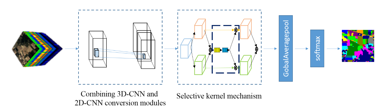
对早年提出的3D-CNN会导致参数量过大,对系统的训练能力要求较强。因此提出了FSKNet解决这一问题。其中主要参考改进点有两个:
- 设计了3D-CNN和2D-CNN转换模块,利用3D-CNN完成特征提取,同时降低空间和光谱的维数。
- 在转换后的2D-CNN中,提出了一种选择性核机制,允许每个神经元根据双向输入信息尺度调整感受野大小。
涉及较新的模型结构
- 2D和3D CNN结合进行特征提取的同时进行降维
- 可变卷积操作
- 可分离卷积操作
- 最后的全局最大池化替换全连接进行加速
网络总体结构
其中所有的网络层结构链接如下表格所示:
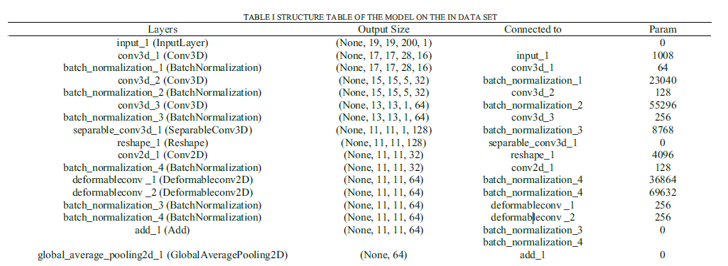
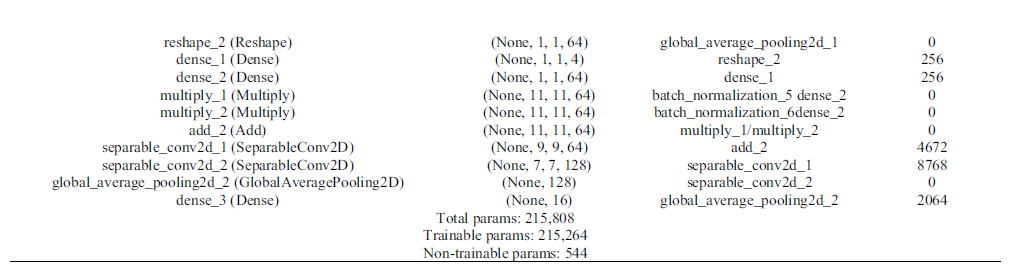
其中给出了所有的层数,输出维度,链接层和参数,接下来将一一阐述。
3D-CNN and 2D-CNN conversion modules
本模块由三层3D-Conv、一层可分离3D-Conv和最后经过reshape操作后的2D-Conv组成:
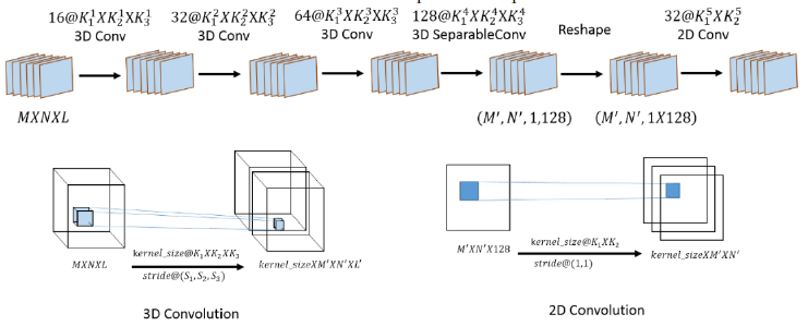
为了避免常规降维时,PCA对其他数据舍弃而导致的信息丢失,本论文采用了一边卷积一边降维的方式,通过设置通道维数的大幅度stride进行降维。
最后通过reshape+2D Conv进行图像的转换防止图像降维。
Selective kernel mechanism
下图是其内部结构:
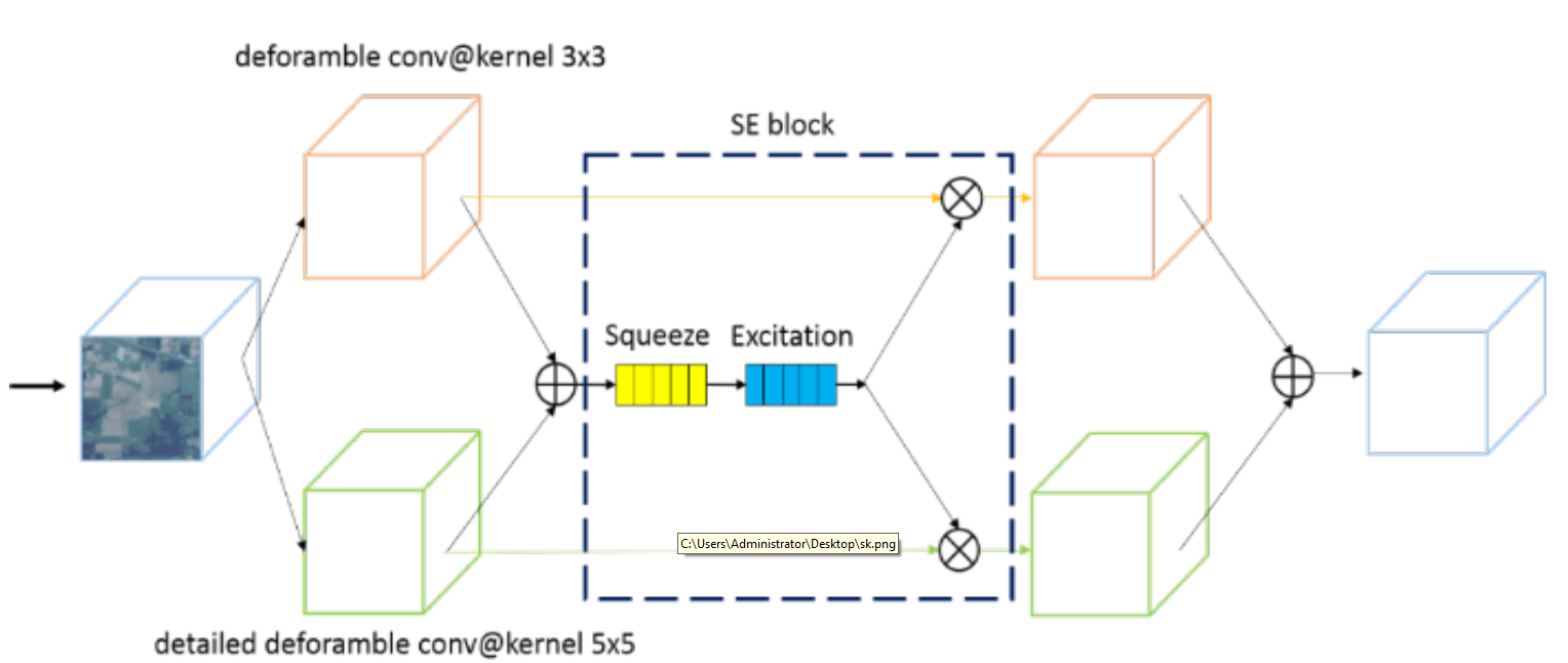
包括了三个重点的结构,可变卷积、注意力机制和可分离卷积。
可变卷积
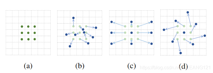
简要概括
可变形卷积是指卷积核在每一个元素上额外增加了一个参数方向参数,这样卷积核就能在训练过程中扩展到很大的范围。
目的
为了解决在采样过程中卷积核过于固定,不能很好的适应局部空间的采样操作。
解决方案
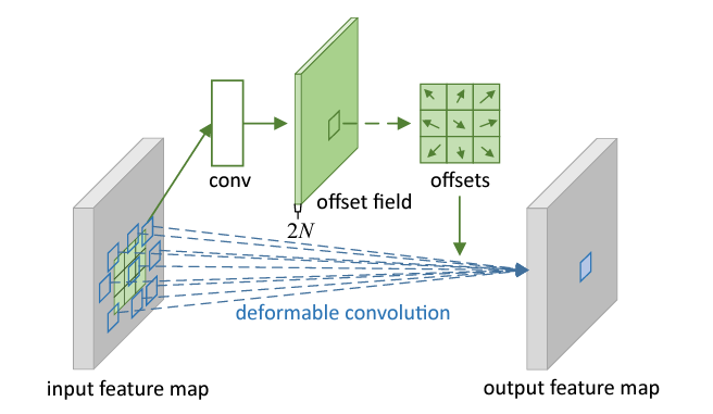
上图是可变形卷积的学习过程,首先偏差是通过一个卷积层获得,该卷积层的卷积核与普通卷积核一样。输出的偏差尺寸和输入的特征图尺寸一致。生成通道维度是2N,分别对应原始输出特征和偏移特征。这两个卷积核通过双线性插值后向传播算法同时学习。
解释
事实上,可变形卷积单元中增加的偏移量是网络结构的一部分,通过另外一个平行的标准卷积单元计算得到,进而也可以通过梯度反向传播进行端到端的学习。加上该偏移量的学习之后,可变形卷积核的大小和位置可以根据当前需要识别的图像内容进行动态调整,其直观效果就是不同位置的卷积核采样点位置会根据图像内容发生自适应的变化,从而适应不同物体的形状、大小等几何形变。然而,这样的操作引入了一个问题,即需要对不连续的位置变量求导。
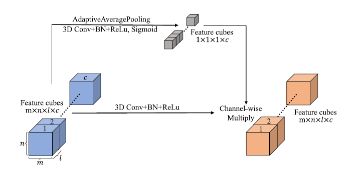
注意力机制
注意力机制主要存在于se block中。
注意力机制主要通过对当前输入的卷积层进行全局平均池化,并使用激活函数对得到的向量进行激活,再乘到相应的卷积层上,以达到对每个卷积层权重的赋值。
可分离卷积
可分离卷积时经过注意力机制之后的卷积操作,通过可分离卷积进行网络加速,达到减小参数量并保持准确率的效果。
分类器部分
通过全局池化操作将上一层的卷积层从7×7×128转换成了长度为128的向量,并通过全卷积降至种类数,进行分类。
代码实现部分
网络结构总体设计:
# 组合模型
class ResnetBuilder(object):
    @staticmethod
    def build(input_shape, num_outputs):
        print('original input shape:', input_shape)
        _handle_dim_ordering()
        if len(input_shape) != 4:
            raise Exception("Input shape should be a tuple (nb_channels, kernel_dim1, kernel_dim2, kernel_dim3)")

        print('original input shape:', input_shape)
        # 根据是否将通道放到最后一维进行变更
        if K.image_dim_ordering() == 'tf':
            input_shape = (input_shape[1], input_shape[2], input_shape[3], input_shape[0])
        print('change input shape:', input_shape)

        input = Input(shape=input_shape)

        # input = applyPCA(input, 30)
        # 3D-CNN and 2D-CNN conversion modules begin
        conv1 = Conv3D(filters=16, kernel_size=(3, 3, 7), strides=(1, 1, 5), kernel_regularizer=regularizers.l2(0.01),
                       kernel_initializer='he_normal', use_bias=False, activation='relu')(input)
        conv1 = BatchNormalization()(conv1)
        conv2 = Conv3D(filters=32, kernel_size=(3, 3, 5), strides=(1, 1, 3), kernel_regularizer=regularizers.l2(0.01),
                       kernel_initializer='he_normal', use_bias=False, activation='relu')(conv1)
        conv2 = BatchNormalization()(conv2)
        print(conv2.shape)
        conv3 = Conv3D(filters=64, kernel_size=(3, 3, 3), strides=(1, 1, 1), kernel_regularizer=regularizers.l2(0.01),
                       kernel_initializer='he_normal', use_bias=False, activation='relu')(conv2)
        conv3 = BatchNormalization()(conv3)
        print(conv3.shape)
        conv3 = SeparableConv3D(filters=128, kernel_size=(3, 3, 1), strides=(1, 1, 1),
                                kernel_initializer=regularizers.l2(0.01),
                                use_bias=False, activation='relu')(conv3)
        print(conv3._keras_shape)
        conv3_shape = conv3._keras_shape

        l = Reshape((conv3_shape[1], conv3_shape[2], conv3_shape[3] * conv3_shape[4]))(conv3)
        print(l)

        # conv11
        l = Conv2D(32, (1, 1), padding='same', kernel_regularizer=regularizers.l2(0.01), kernel_initializer='he_normal',
                   use_bias=False, activation='relu')(l)
        l = BatchNormalization()(l)
        print(l.shape)
        # 3D-CNN and 2D-CNN conversion modules end

        # Selective kernel mechanism begin
        # conv12 - 可变卷积
        l_offset = ConvOffset2D(32)(l)  # 求取偏移量offset
        l1 = Conv2D(64, (3, 3), padding='same', strides=(1, 1), kernel_regularizer=regularizers.l2(0.01),
                    kernel_initializer='he_normal', use_bias=False, activation='relu')(l_offset)
        l1 = BatchNormalization()(l1)
        print(l1.shape)

        # conv21 - 可变卷积
        l_offset = ConvOffset2D(32)(l)  # 求取偏移量offset
        l2 = Conv2D(64, (5, 5), padding='same', strides=(1, 1), dilation_rate=5,
                    kernel_regularizer=regularizers.l2(0.01), kernel_initializer='he_normal', use_bias=False,
                    activation='relu')(l_offset)
        l2 = BatchNormalization()(l2)
        print(l2.shape)

        l = keras.layers.add([l1, l2])
        # attention 操作
        se = squeeze_excite_block(l)
        l1 = multiply([l1, se])
        l2 = multiply([l2, se])

        l = keras.layers.add([l1, l2])
        print(l)
        # 可分离卷积
        l = SeparableConv2D(filters=128, kernel_size=(3, 3), strides=(1, 1), kernel_initializer=regularizers.l2(0.01),
                            use_bias=False, activation='relu')(l)
        l = BatchNormalization()(l)
        l = SeparableConv2D(filters=256, kernel_size=(3, 3), strides=(1, 1), kernel_initializer=regularizers.l2(0.01),
                            use_bias=False, activation='relu')(l)
        l = BatchNormalization()(l)
        # Selective kernel mechanism end
        # out
        l = GlobalAvgPool2D()(l)

        # 输入分类器
        # Classifier block
        dense = Dense(units=num_outputs, activation="softmax", kernel_initializer="he_normal")(l)

        model = Model(inputs=input, outputs=dense)
        return model

    @staticmethod
    def build_resnet_8(input_shape, num_outputs):
        # (1,7,7,200),16
        return ResnetBuilder.build(input_shape, num_outputs)
数据准备:
# 加载数据
mat_data = sio.loadmat('F:/transfer code/Tensorflow  Learning/SKNet/datasets/IN/Indian_pines_corrected.mat')
data_IN = mat_data['indian_pines_corrected']
# 标签数据
mat_gt = sio.loadmat('F:/transfer code/Tensorflow  Learning/SKNet/datasets/IN/Indian_pines_gt.mat')
gt_IN = mat_gt['indian_pines_gt']
# print('data_IN:',data_IN)
print(data_IN.shape)
# (145,145,200)
print(gt_IN.shape)
# (145,145)
# 标签拷贝
new_gt_IN = gt_IN

batch_size = 16

nb_classes = 16
nb_epoch = 200  # 400
# 单个训练样本长宽大小
img_rows, img_cols = 23, 23  # 27, 27
patience = 200


INPUT_DIMENSION_CONV = 200
INPUT_DIMENSION = 200

TOTAL_SIZE = 10249
VAL_SIZE = 1025

TRAIN_SIZE = 5128
TEST_SIZE = TOTAL_SIZE - TRAIN_SIZE
VALIDATION_SPLIT = 0.5  # 20% for training and 80% for validation and testing
# 0.9  1031
# 0.8  2055
# 0.7  3081
# 0.6  4106
# 0.5  5128
# 0.4  6153

# 通道数
img_channels = 200
PATCH_LENGTH = 11  # Patch_size (13*2+1)*(13*2+1)

print(data_IN.shape[:2])
# (145,145)
print(np.prod(data_IN.shape[:2]))
# 21025
print(data_IN.shape[2:])
# (200,)
print(np.prod(data_IN.shape[2:]))
# 200
print(np.prod(new_gt_IN.shape[:2]))
# 21025

# 对数据进行reshape处理之后,进行scale操作
data = data_IN.reshape(np.prod(data_IN.shape[:2]), np.prod(data_IN.shape[2:]))
gt = new_gt_IN.reshape(np.prod(new_gt_IN.shape[:2]), )

# 标准化操作,即将所有数据沿行沿列均归一化道0-1之间
data = preprocessing.scale(data)
print(data.shape)
# (21025, 200)

# 对数据边缘进行填充操作,有点类似之前的镜像操作
data_ = data.reshape(data_IN.shape[0], data_IN.shape[1], data_IN.shape[2])
whole_data = data_
padded_data = zeroPadding.zeroPadding_3D(whole_data, PATCH_LENGTH)
print(padded_data.shape)
# (151, 151, 200)
# 因为选择的是7*7的滑动窗口,145*145,145/7余5,也就是说有5个像素点扫描不到,所有在长宽每边个填充3,也就是6,这样的话
# 就可以将所有像素点扫描到

ITER = 1
CATEGORY = 16
# 提前准备训练集的接收格式
train_data = np.zeros((TRAIN_SIZE, 2 * PATCH_LENGTH + 1, 2 * PATCH_LENGTH + 1, INPUT_DIMENSION_CONV))
print(train_data.shape)
# 提前准备测试集的接收格式
test_data = np.zeros((TEST_SIZE, 2 * PATCH_LENGTH + 1, 2 * PATCH_LENGTH + 1, INPUT_DIMENSION_CONV))
print(test_data.shape)

# 评价指标
KAPPA_3D_HSICNNet = []
OA_3D_HSICNNet = []
AA_3D_HSICNNet = []
TRAINING_TIME_3D_HSICNNet = []
TESTING_TIME_3D_HSICNNet = []
ELEMENT_ACC_3D_HSICNNet = np.zeros((ITER, CATEGORY))

# seeds = [1220, 1221, 1222, 1223, 1224, 1225, 1226, 1227, 1228, 1229] 随机数种子
seeds = [1334]
训练步骤:
for index_iter in range(ITER):
    print("# %d Iteration" % (index_iter + 1))
    # Iteration

    # save the best validated model
    best_weights_HSICNNet_path = 'F:/transfer code/Tensorflow  Learning/SKNet/models-in-densenet-23-514/Indian_best_3D_HSICNNet_' + str(
        index_iter + 1) + '.hdf5'

    # 通过sampling函数拿到测试和训练样本
    np.random.seed(seeds[index_iter])
    train_indices, test_indices = sampling(VALIDATION_SPLIT, gt)
    # train_indices 2055     test_indices 8094

    # gt本身是标签类,从标签类中取出相应的标签 -1,转成one-hot形式
    y_train = gt[train_indices] - 1
    y_train = to_categorical(np.asarray(y_train))

    y_test = gt[test_indices] - 1
    y_test = to_categorical(np.asarray(y_test))
    # whole_data 是未填充之前的图片、train_indices是用做训练的训练点。
    train_assign = indexToAssignment(train_indices, whole_data.shape[0], whole_data.shape[1], PATCH_LENGTH)
    for i in range(len(train_assign)):
        train_data[i] = selectNeighboringPatch(padded_data, train_assign[i][0], train_assign[i][1], PATCH_LENGTH)
    # whole_data 是未填充之前的图片、train_indices是用做训练的训练点。
    # 返回的是在整个数据图片上的x,y坐标对
    test_assign = indexToAssignment(test_indices, whole_data.shape[0], whole_data.shape[1], PATCH_LENGTH)
    for i in range(len(test_assign)):
        # 求取该像素点周围预设卷积区域的大小
        test_data[i] = selectNeighboringPatch(padded_data, test_assign[i][0], test_assign[i][1], PATCH_LENGTH)

    x_train = train_data.reshape(train_data.shape[0], train_data.shape[1], train_data.shape[2], INPUT_DIMENSION_CONV)
    x_test_all = test_data.reshape(test_data.shape[0], test_data.shape[1], test_data.shape[2], INPUT_DIMENSION_CONV)
	# 选取部分进行训练
    x_val = x_test_all[-VAL_SIZE:]
    y_val = y_test[-VAL_SIZE:]
	# 选取部分进行测试
    x_test = x_test_all[:-VAL_SIZE]
    y_test = y_test[:-VAL_SIZE]
	# 加载模型
    model_HSICNNet = model_HSICNNet()

    # 创建一个实例history
    history = LossHistory()

    # monitor:监视数据接口,此处是val_loss,patience是在多少步可以容忍没有提高变化
    earlyStopping6 = kcallbacks.EarlyStopping(monitor='val_loss', patience=patience, verbose=1, mode='auto')
    # 用户每次epoch最后都会保存模型,如果save_best_only=True,那么最近验证误差最后的数据将会被保存下来
    saveBestModel6 = kcallbacks.ModelCheckpoint(best_weights_HSICNNet_path, monitor='val_loss', verbose=1,
                                                save_best_only=True,
                                                mode='auto')

    # 训练和验证
    tic6 = time.clock()
    print(x_train.shape, x_test.shape)
    # (2055,7,7,200)  (7169,7,7,200)
    history_3d_HSICNNet = model_HSICNNet.fit(
        x_train.reshape(x_train.shape[0], x_train.shape[1], x_train.shape[2], x_train.shape[3], 1), y_train,
        validation_data=(x_val.reshape(x_val.shape[0], x_val.shape[1], x_val.shape[2], x_val.shape[3], 1), y_val),
        batch_size=batch_size,
        nb_epoch=nb_epoch, shuffle=True, callbacks=[earlyStopping6, saveBestModel6, history])
    toc6 = time.clock()

    # 测试
    tic7 = time.clock()
    loss_and_metrics = model_HSICNNet.evaluate(
        x_test.reshape(x_test.shape[0], x_test.shape[1], x_test.shape[2], x_test.shape[3], 1), y_test,
        batch_size=batch_size)
    toc7 = time.clock()

    print('3D HSICNNet Time: ', toc6 - tic6)
    print('3D HSICNNet Test time:', toc7 - tic7)

    print('3D HSICNNet Test score:', loss_and_metrics[0])
    print('3D HSICNNet Test accuracy:', loss_and_metrics[1])

    print(history_3d_HSICNNet.history.keys())

    # 预测
    pred_test = model_HSICNNet.predict(
        x_test.reshape(x_test.shape[0], x_test.shape[1], x_test.shape[2], x_test.shape[3], 1)).argmax(axis=1)
    # 跟踪值出现的次数
    collections.Counter(pred_test)

    gt_test = gt[test_indices] - 1
    # print(len(gt_test))
    # 8194
    # 这是测试集,验证和测试还没有分开
    overall_acc = metrics.accuracy_score(pred_test, gt_test[:-VAL_SIZE])
    confusion_matrix = metrics.confusion_matrix(pred_test, gt_test[:-VAL_SIZE])
    each_acc, average_acc = averageAccuracy.AA_andEachClassAccuracy(confusion_matrix)
    kappa = metrics.cohen_kappa_score(pred_test, gt_test[:-VAL_SIZE])
    KAPPA_3D_HSICNNet.append(kappa)
    OA_3D_HSICNNet.append(overall_acc)
    AA_3D_HSICNNet.append(average_acc)
    TRAINING_TIME_3D_HSICNNet.append(toc6 - tic6)
    TESTING_TIME_3D_HSICNNet.append(toc7 - tic7)
    ELEMENT_ACC_3D_HSICNNet[index_iter, :] = each_acc

    # 绘制acc-loss曲线
    history.loss_plot('epoch')

    print("3D HSICNNet finished.")
    print("# %d Iteration" % (index_iter + 1))
运行环境:
python3.7 + tensorflow1